College Senior Project
Hash Grid and Screen-Space Tile Photon Gathering in 3D Interactive Applications
NOTE: This is also available via the DIGITAL COMMONS @ CAL POLY
ABSTRACT
This project is an exploration of GPU programming that implements two photon mapping pipelines based on the work of Mara et. al [5] and Singh et. al [6] to achieve interactive rendering performance for a set of simple scenes. In particular, 3D hash grid and screen-space tiling algorithms are used to accelerate photon lookup to compute direct and indirect lighting on visible surfaces in a scene. Users who rely on complex lighting situations, such as in CAD and movie production, would use this kind of system to more quickly and effectively evaluate how their scenes and models will appear in a final rendering.
1. INTRODUCTION
Modern rendering algorithms utilize multicore computation devices, typically GPUs, to accelerate pixel color computations in a resulting image. The application programmer interfaces (APIs) that expose access to these devices are complex and merit a great deal of specialized knowledge and experience in order to utilize them effectively for rendering. The main object of this project is to simultaneously gain experience with a particular API, namely OpenCL, and how it can be used to implement rendering techniques that are near the forefront of current raytracing research.
Raytracing can be used to realistically render scenes with high visual complexity but at huge computational cost. For users of CAD applications and in movie production who work on scenes where visual realism is required, final renders take a substantial period of time to produce acceptable results. However, engineers, artists, and designers creating objects and scenes need a good sense of how the image or scene will look given a complex set of object properties and lighting conditions as they are creating them. By using photon mapping techniques in conjunction with GPU programming, fast and reasonable approximations can be delivered to these users at an interactive rate (~500ms or 2 frames per second) to both speed up work flows and decrease the time of final renders.
2. BACKGROUND & RELATED WORK
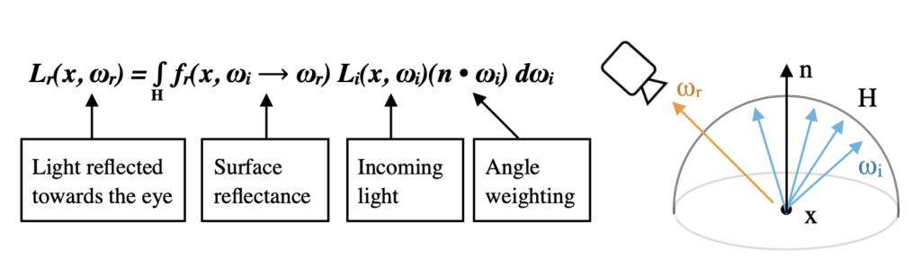
Scenes are rendered by using a combination of mathematical descriptions of object surfaces and how light is perceived at visible surface points by a viewer. The rendering equation, as shown in Figure 1, describes how light reflected towards the viewer, Lr, is the sum of the product of the surface reflectance, fr, and incoming light, Li, weight by the angle formed by the surface normal n, over the hemisphere H, around a visible surface point x, given the vector to the viewer ωr.
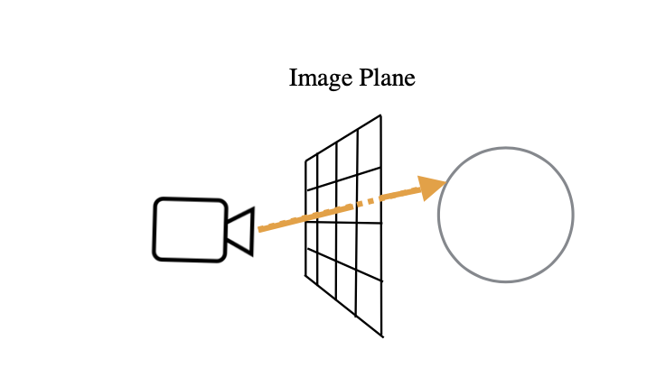
One way of generating an image using the rendering equation is by raytracing. In general, raytracing involves splitting a camera’s field of view into a uniform grid of pixels and then tracing rays from the camera, through the center of those pixels, and into the scene, as shown in Figure 2. The color of each visible surface hit by a particular ray is then determined by the rendering equation shown in Figure 1.
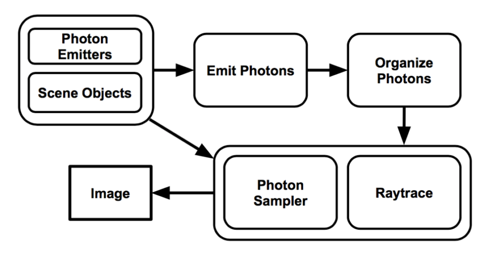
Figuring out the incoming light, or irradiance, requires knowledge of how light interacts with the scene and makes its way to the surfaces to be rendered. Irradiance can be approximated using a photon map. Using photon maps to approximate irradiance and global illumination effects was first introduced by Henrik Wann Jensen in 1996. According to Jensen, a photon map is constructed by “emitting photons from light sources in the model and storing these in the photon map as they hit surfaces,” eventually creating “a rough representation of the light within the scene.” This photon map is then sampled to determine the lighting at surface points with respect to the viewer [4]. This photon mapping pipeline is summarized in Figure 3 and discussed further in Section 3.
In general, photon mapping is a good candidate for robust and interactive rendering (0.2-1.0s) because it captures a wide range of global illumination visual effects and scales very well as multicore hardware becomes more powerful [5]. This project relies heavily on the work of Singh et. al and their project “Photon Mapper” which implements an interactive, progressive hash grid photon mapping raytracer built using CUDA [6] and the work of Mara et. al and their survey of different algorithms, including a screen-space tiling algorithm, for accelerating photon mapping using CUDA [5]. Each of these use the GPU to parallelize the work of their raytracers.
Raytracers are relatively simple to parallelize on a per-ray basis provided that a ray trace does not change the scene and writes to a pixel independently of others [7]. However, for optimizing a parallel implementation memory alignment and buffer size matching cache lanes on the GPU must be considered, as well as using float computations instead of integers ones whenever possible [3], using as little kernel memory as possible, and working over larger datasets [1]. This fine grain control is not explicitly present in OpenGL and DirectX, and so APIs like OpenCL, CUDA, Vulcan, and Metal have been created to provide the necessary interfaces for creating and optimizing parallelized code.
Unlike Singh and Mara, who use CUDA, this project utilizes OpenCL, a cross-platform parallel programming system, in order to implement the parallelized raytracing pipeline. APIs like Metal, which are locked to platform, and CUDA, which are locked to specific hardware, limit the scope of where parallel computing solutions can be applied and who gets access to these solutions.
3. ALGORITHM & IMPLEMENTATION
As shown in Figure 3, a photon mapping pipeline utilizes a scene description to emit photons, to organize photons, and then to raytrace the scene. The hash grid and tiling methods modify how photons are organized and sampled to accelerate the raytracing step.
This biggest challenge for this project, beyond understanding the photon mapping pipeline, was organizing key algorithms into OpenCL kernels, and communicating information about the scene and each step to the host CPU and to other OpenCL kernels. OpenCL 1.2’s kernel language, which was used to write almost all of the algorithms, is a subset of C, does not support recursive function calls, and does not support dynamic memory allocation. The consequences of these limitations will be discussed throughout the following sections.
3.1 SCENE DATA REPRESENTATION
Point lights, planes, and spheres where the only types of scene objects that were represented, mainly to simplify intersection testing and keep the project focused on correctness.
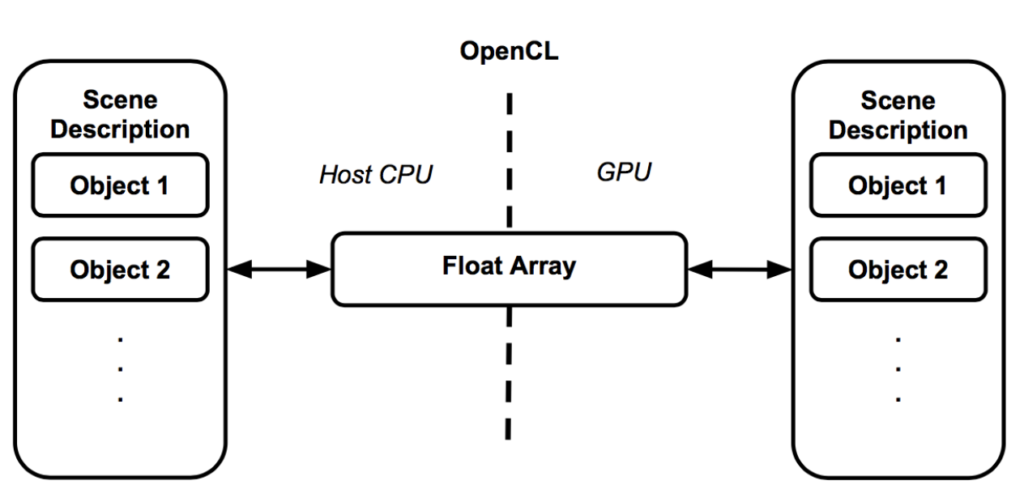
Since OpenCL is designed to work with any number of different computation devices, there is no strict guarantee that structs in an OpenCL kernel will match the same data layout as on the host CPU (there is a packed attribute that can be applied but the OpenCL compiler used did not properly support it). So scene objects on the host device would be placed into a float array, sent off to the compute device, and then recreated as needed during execution, as shown in Figure 4.
3.2. PHOTON EMISSION & SAMPLING
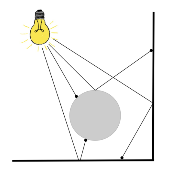
Photon maps are constructed by “emitting a large number of photons (packets of energy) from the light sources in the scene” [4]. As stated before, this project only considers point lights when mapping photons into the scene. Photons are given an equal portion of their source light’s energy when they are emitted and as they bounce the photons alter their energy using the surface properties of the objects they have hit. As a photon strikes a surface, Russian roulette [2] is used to determine if the photon bounces off into the scene and further hit tests must be performed. Figure 6 shows the result of emitting photons into a sample 2D scene.
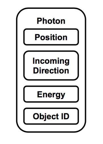
Photons are represented using the position of where the photon has stopped bouncing, a normalized incoming direction of where the photon was headed when it stopped on the surface, an RGB energy, and the ID of the object that the photon has stopped on, as shown in Figure 5. Because there is no dynamic memory allocation explicitly supported in OpenCL kernels, a fixed size array is allocated to store all the resulting emitted photons. If a photon does not stick onto any surfaces, the kernel will simply keep emitting photons until all slots in the photon array are filled.
Once a photon map is constructed we collect a sample of photons around surface points and use them to estimate the direct and indirect illumination at each point. While a K-nearest neighbors algorithm was first used to find a representative sample of photons at surface points [4], the final implementation uses photon effect radii [5]. In practice, K-nearest neighbors required that each kernel have its own chunk of K slots of memory available for keeping a priority queue of the nearest photons. This extra memory often proved to far exceed what was available to each kernel and placed a memory bottleneck on the application.
By contrast, with uniform photon effect radii every visible surface point gets an equal spatial chunk of photons allowing for both consistent results when shading and far less memory usage per ray cast, but also for shadows to naturally emerge from regions that are less dense in photons. The result of using uniform effect radii is that when sampling photons we do so in a sphere around the visible surface point.
3.2. 3D HASH GRID
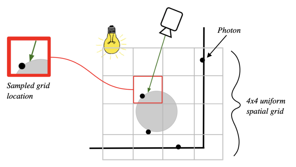
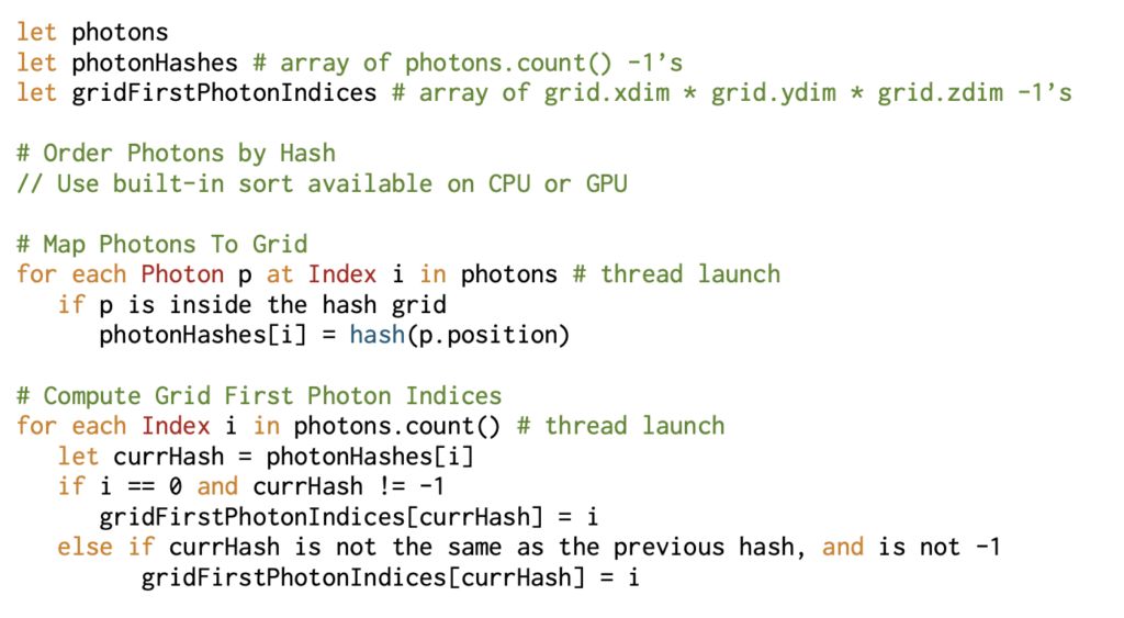
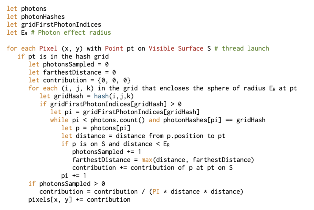
The 3D hash grid algorithm works by sorting sorting photons in the photon map by their grid location (spatial hash) and then only sampling photons that are within a uniform photon effect radius ER of the visible surface point, using the spatial grid to limit the search to nearby photons. Figure 7 shows an example of using a 2D hash grid and Listing 1 and Listing 2 in Appendix A describe the steps to build and traverse the spatial hash.
The main drawbacks of this approach are that only photons within the grid can be queried and used for sampling, that all the photons in the scene must be passed to every kernel, and that the extra data for the grid can be a data bottleneck for higher resolution grids. For static scenes a hash grid is ideal because placing photons into the grid can be expensive, but searching the grid generally is not. As with Figure 7, the 4×4 2D grid shown only covers a specific area of the scene and so only photons within this space can be searched and collected.
In Listing 1 and Listing 2, the variables photonHashes and gridFirstPhotonIndices are global data arrays that store the information of the hash grid. Since OpenCL does not have a builtin sort function, the photons were sorted on the CPU using C++’s std::sort function. Once sorted, each photonHashes[i] is initialized to the hash of each corresponding photons[i]. Each gridFirstPhotonIndices[j] stores the first time j occurs in photonHashes, or else some default “no first index” value such as -1. Thus a non-negative gridFirstPhotonIndices[j] indicates there are some photons at that grid location. Notice that since photons are sampled in a uniform sphere, the hash grid only needs to be sampled in the grid spaces that touch the sphere.
3.3. SCREEN-SPACE TILING
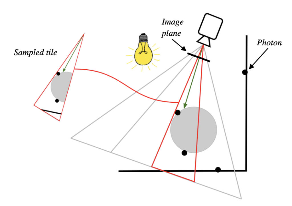
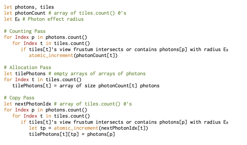
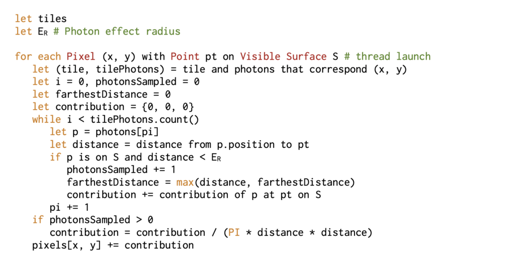
The screen-space tiling algorithm works by grouping rectangles of pixels together into tiles. Then every render frame the tile’s view frustum is used to place photons into buckets when they are within ER of the view frustum. When rendering the scene, only the photons for the current tile are sampled since they are guaranteed to be within the sampling sphere for any particular visible surface in the tile. Figure 8 shows an example of a 2D tiling algorithm in action, and Listing 3 and Listing 4 of Appendix B describe the steps of how to fill and use the tiles.
Although this algorithm requires that the photons be placed into tiles every single render frame, scenes that add and remove photons dynamically require no special handling for the tiling method. In practice, the tiling step is about thirty times faster than the tile sampling step, and so does not present a significant bottleneck to performance. The present implementation does not cull photons that are behind other objects within the tile frustum leading to excess photons being left for the sampling step for scenes of large depth variance.
As described in Listing 3 and Listing 4, tile construction works by first counting how many photons belong into each tile, then allocating enough space for each tile’s photons, and finally placing the photons into each tile. This structure for the algorithm is great for GPUs since allocation must be done on the CPU anyways and that a single photon can be worked on by its own kernel without lots of data fetches.
4. RESULTS
This project focused on how to use a parallelization API like OpenCL to implement a photon mapping pipeline for raytracing. So while there will be a coarse analysis of the parallelized implementations, there will also be a look at how to use the ideas and techniques learned from working with OpenCL and applying them to OpenGL.
4.1 SINGLE CORE AND OPENCL
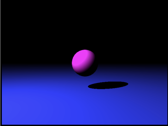
Figure 9: Two colored light sources Photons using Direct ray tracing 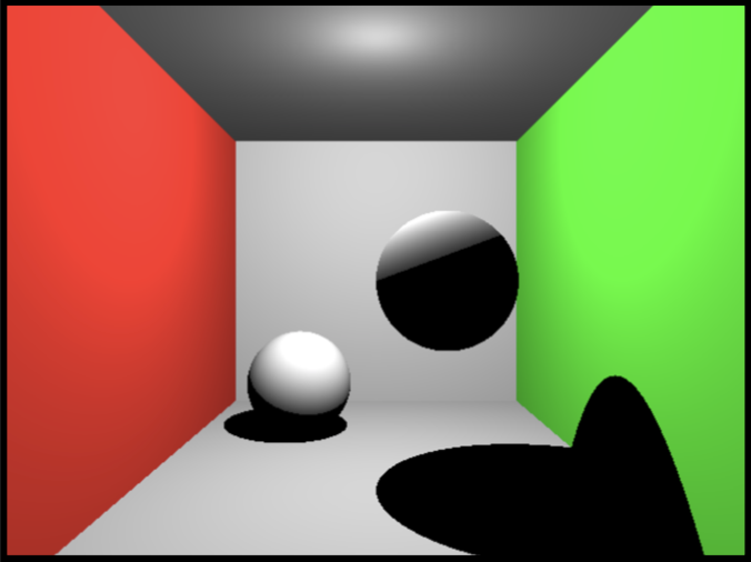
Figure 10: Two colored light sources Photons using Direct ray tracing 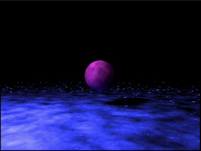
Figure 11: sphere_and_plane with 12k Photons using Screen-Space Tiling 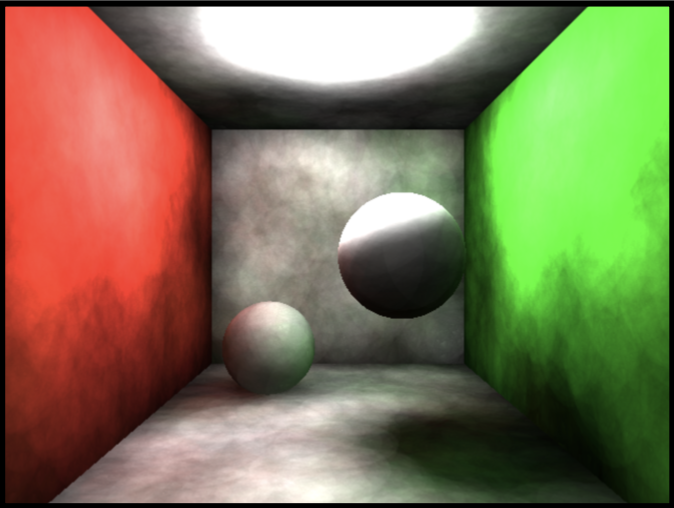
Figure 12: GIRefScene with 12k Photons using Screen-Space Tiling 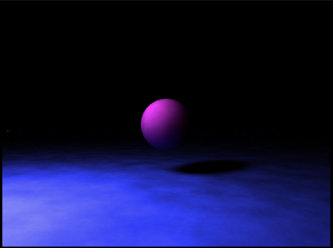
Figure 13: sphere_and_plane with 200k Photons using Screen-Space Tiling 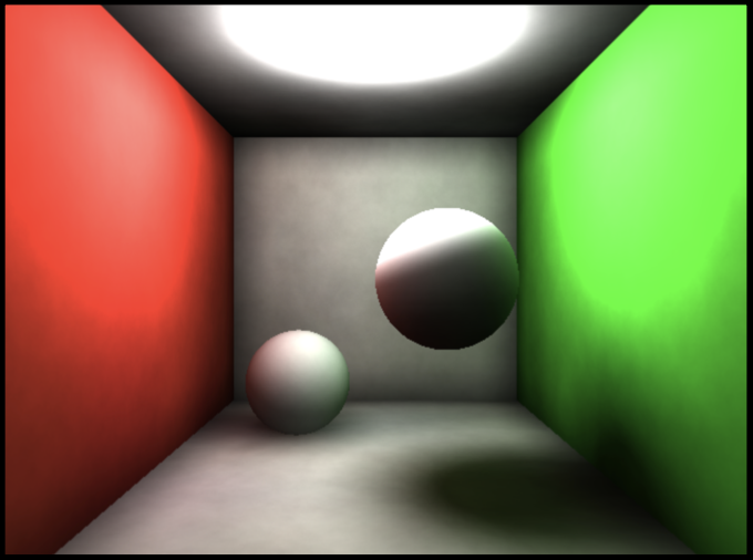
Figure 14: GIRefScene with 200k Photons using Screen-Space Tiling 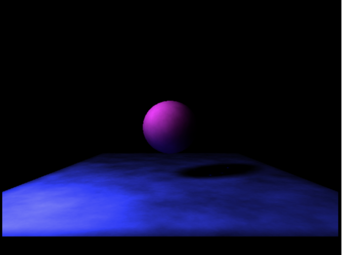
Figure 15: sphere_and_plane 200k Photons using Hash Grid 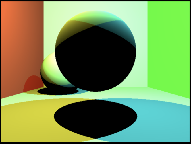
Figure 16: Two colored light sources Photons using Direct ray tracing 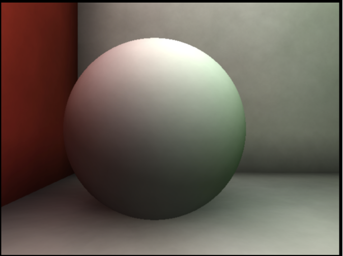
Figure 17: Color bleeding from walls 200k Photons using Screen-Space Tiling 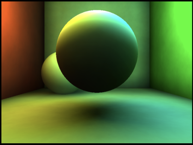
Figure 18: Two colored light sources 200k Photons using Screen-Space Tiling
The final product includes six different ray tracers, each with its own unique combination of algorithm (direct illumination/hash grid/tiling) and computing architecture (single-threaded/ OpenCL). The single-threaded implementation ran on a 2.3 GHz Intel Core i7 and then the massively parallel implementation on an NVIDIA GeForce GT 650M. These raytracers where written all in C++11 with GPU kernels written in OpenCL 1.2.
Figures 9 and 10 rendered the two principal scenes GIRefScene (an abbreviation of “Global Illumination Reference Scene”) and sphere_and_plane using a simplified direct raytracer where the color of the surface does not take into account irradiance of the scene (other than if there is a direct path to the light) at 640 by 480 pixels. These renders, which rendered in realtime, give a baseline time for figuring out the visible surfaces as well as what basic features the scenes should have, such as shadow placement, light glare, and object placement and color.
Figures 11 and 13 show the scene sphere_and_plane rendered at 640×480 using the tiling algorithm with 12k and 200k photons respectively. The scene if composed of a point light source, a sphere, and a plane. Half of the scene is complete darkness since there are no objects above the sphere, leading to significantly higher draw rates for the scene in general. Since sphere_and_plane is not bounded on all sides like with GIRefScene, notice the white speckles that lie at the edge of where the light is least intense. As parts of the scene farther from the light are rendered, the level of error in irradiance calculation increases. This can be mitigated by increasing the number of photons, as is evident in Figure 13.
For the most part, using a hash grid and tiling produce identical results when rendering parts of the scene within the bounds of the hash grid. However, as shown in Figure 15, when the rendered view exceeds the extent of the hash grid scene nothing can be rendered. So while sphere_and_plane cannot easily escape this problem, GIRefScene has a finite region of interest for rendering in the scene.
Figures 12 and 14 show the scene GIRefScene rendered at 640×480 using the tiling algorithm with 12k and 200k photons respectively. The scene is composed of a point light source just below the ceiling, six planes, and two spheres, with only the left and right planes’ surface colors being other than grey. This scene acted as the main benchmark for ensuring correctness for the algorithms but also performance of each algorithm. Since photons are bounced around a bounded space, the scene generally has better visual results than with unbounded scenes such as sphere_and_plane.
Figures 16 and 18 show off the renderer using two point lights of different color. The point light on the left is a yellowish light, and the one on the right is a blueish light. Adding lights to a photon mapping system requires no additional effort other than for those new lights to emit their own photons at the photon emission step. For this implementation, additional lights are given a random subset of the total number of photons in order to keep the amount of energy in the scene the same. Note how the plane beneath the central sphere exhibits the differently colored shadows blending and that the left and right sides take on the color of the light with a direct path to that surface.
Figures 17 and 18 show some of the benefits to using photon maps to calculate irradiance and, in turn, soft shadows and color bleeding. Soft shadows are generated as the result of photon density varying due to how much of the rendered surface is effected by the light and surrounding objects. Similarly, as photons bounce from one part of the scene to another, the light from some objects, like the wall to the left of the sphere in Figure 17, contribute to the color of the objects that are rendered, hence color bleeding.
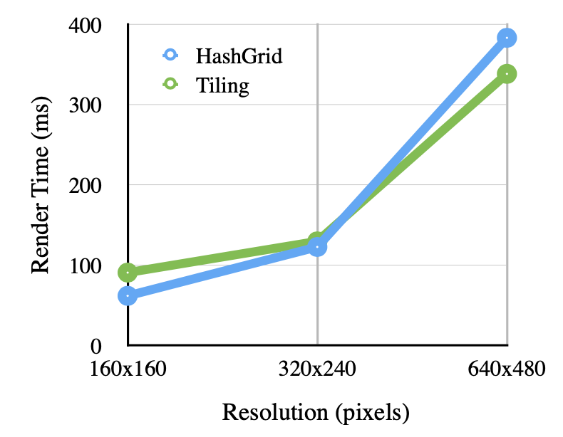
Graph 1: Render times for OpenCL HashGrid and Tiling for GIRefScene 12k Photons 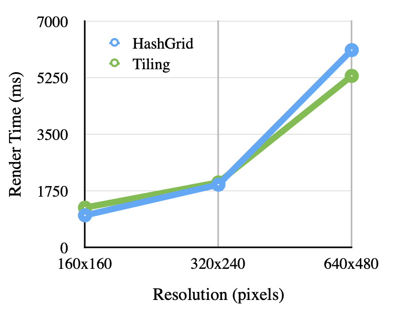
Graph 2: Render times for OpenCL HashGrid and Tiling for GIRefScene 200k Photons 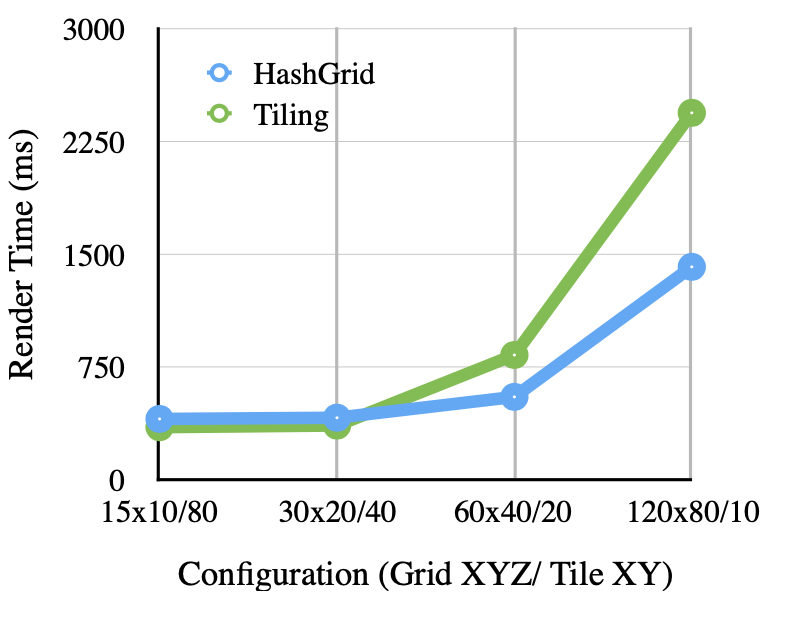
Graph 3: Render times for OpenCL HashGrid and Tiling for sphere_and_plane 12k Photons 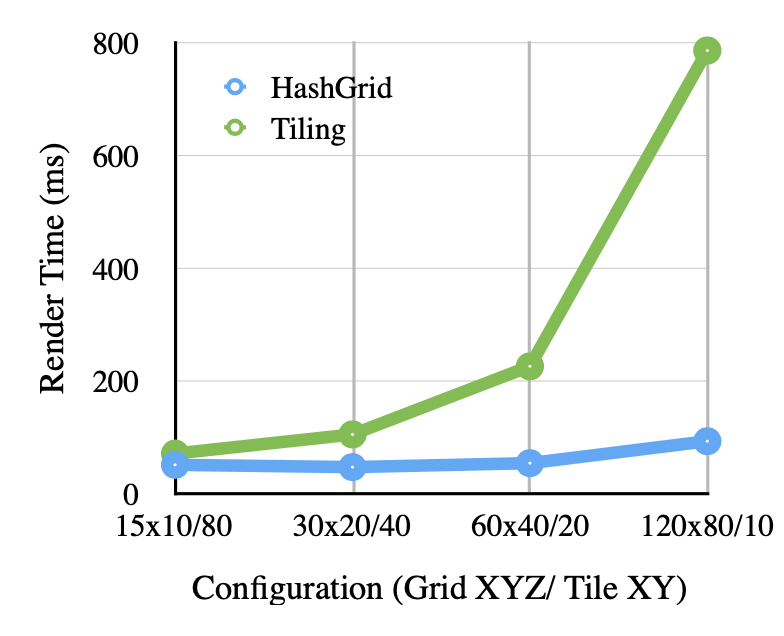
Graph 4: Render times for OpenCL HashGrid and Tiling for sphere_and_plane 200k Photons 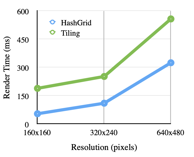
Graph 5: Render times for OpenCL HashGrid and Tiling for sphere_and_plane 12k Photons over various grid and tile configurations 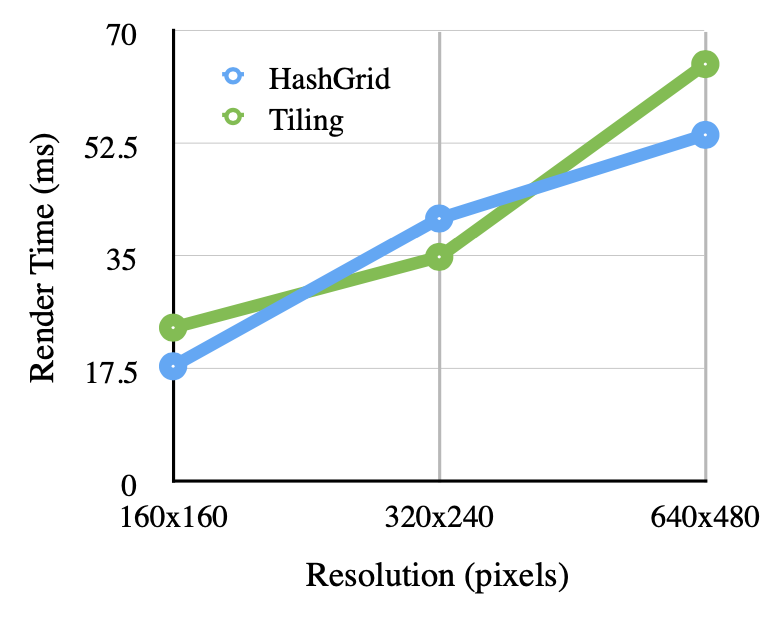
Graph 6: Render times for OpenCL HashGrid and Tiling for GIRefScene12k Photons over various grid and tile configurations
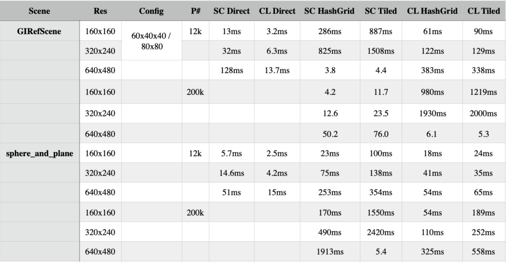
Graphs 1 through 4 show the speed comparison for rendering GIRefScene and sphere_and_plane with the hash grid keeping a fixed 60x40x40 grid and 80×80 pixels being gathered into tiles. In this implementation, the performances tradeoffs between each method depended heavily on the contents of the scene. In general, with the configurations of the tiles and grid are a good fit for the scene to be rendered, the render times do not usually differ by more than 20%. While the tiling method tended to have an edge over the hash grid in GIRefScene as resolution increased, the opposite was true for the simpler sphere_and_plane scene. Under most circumstances when photons were kept reasonably under 200k the scenes tested always had a lowest render time that was still interactive.
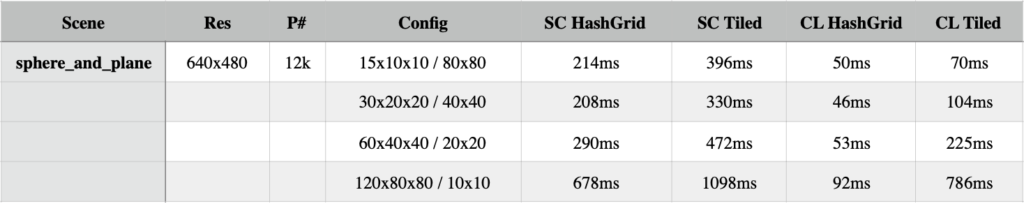
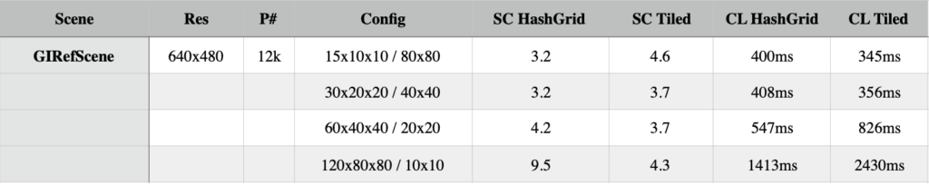
Finally, Graphs 5 and 6 detail the render times for tiling and the grid approach under various configurations for the sphere_and_plane scene and GIRefScene, respectively. The x-axis shows increasing density of the data structures, from 1,500 to 768,000 grid slots and 48 to 3,072 tiles. In general for the both scenes the hash grid did not see a significant performance hit in comparison to tiling. Under the current implementation, it does appear that the hash grid, despite being limited with respect to where rendering can take place in a scene, does prove to more robust than screen-space tiling under very different configurations of the data structure.
4.2 RAYTRACING AND OPENGL
OpenGL is a cross-platform 3D graphics API to work with the GPU. Typically its domain is limited to rasterized graphics. However, OpenGL (> 3.2) can be used to perform raytracing, as laid out in Figure 19. Creating a raytracer using OpenGL is not new, but here acts more of an exercise of using the same techniques, namely data packing and unpacking, to leverage this API to parallelize a rendering algorithm that is not rasterization.
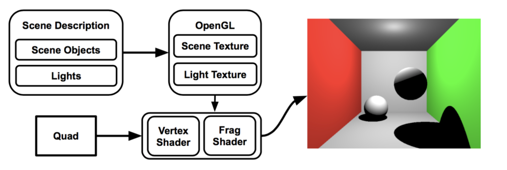
The two main steps that are not entirely obvious involve generating rays and then giving every pixel access to the scene representation. For ray generation, a quad from (-1.0, -1.0, 0.0) to (1.0, 1.0, 0.0) is rendered with texture coordinates (0.0, 0.0) on the bottom left and (1.0, 1.0) at the top right. The vertex shader simply passes on the provided texture coordinate to the fragment shader. In the fragment shader the texture coordinate has now been interpolated and can be thought to be pointing to the pixel that should be rendered. Using the texture coordinate and the camera’s basis vectors, a ray is created that points to the center of each pixel in the image plane.
Scene objects and lights can be accessed in the fragment shader by packing them into a texture. This can be done by first determining how objects should be laid out as a series of floats. For example, a sphere and plane need four floats to give basic geometric information (radius and position for a sphere, normal and distance along the normal for a plane), seven floats for lighting information (color, ambient, diffuse, specular, roughness), and a float for type (sphere or plane type). If each pixel in the texture only has three float components per texture, then a single object would fit into four pixels evenly. In order for float values beyond 0 and 1 to be used in the texture an internal format of GL_RGBF32 must be used so that the values will not be clamped when loaded into the texture.
In the fragment shader, where the scene objects and lights will be reconstructed, the texture’s width and height must be made available so that the center of each texel can be accurately sampled. Object reconstruction occurs by reading in the line of pixels that make up an object and then reading out the float components to each corresponding property of the object. With the objects reconstructed, the entire raytracing pipeline is left entirely unchanged.
Surprisingly, this OpenGL raytracer runs with almost identical performance to the OpenCL direct raytracer discussed earlier in Section 4.1. This OpenGL raytracer was built over a weekend and shows how useful learning OpenCL was to making creative and effective use of a different parallelization API.
5. FUTURE WORK
The presented implementation focused mainly on building an interactive rendering pipeline for simple scenes using direct and indirect lighting. However, most ray tracers also support refraction, reflections, caustics, antialiasing and use ray tracing acceleration structures such as a bounding volume hierarchy (BVH). Both the hash grid and tiling algorithms can be extended to support these features and accelerated using different techniques. Since GPUs tend to be memory bound, integrating a BVH to cull out objects that will be not be rendered as well as integrating a z-buffer to incrementally update the initial closest intersections would help the ray tracing algorithms support larger and more complicated scenes.
As implemented, screen-space tiling would need to be extended in order to support gathering photons for rays that reflect and refract off of different surfaces during the raytracing process. Additionally, screen-space tiling can be accelerated by culling off excess photons not needed during the photon sampling step by using a depth buffer.
The hash grid algorithm can be extended to use a more advanced search along the gradient of the surface being sampled. By limiting the search to gradient, only grid spaces that contain the surface will be searched instead of other nearby objects and empty space. And finally, it may be fruitful to hybridize photon tiling with the hash grid method where photons are sorted on a per tile basis into a hash grid bounded by the tile’s frustum.
6. REFERENCES
[1] APPLE. 2013. Tuning Performance On the GPU. Online: https://developer.apple.com/library/mac/documentation/Performance/Conceptual/OpenCL_MacProgGuide/TuningPerformanceOntheGPU/TuningPerformanceOntheGPU.html
[2] ARVO, J. and KIRK, D. “Particle Transport and Image Synthesis”. Computer Graphics 24 (4), pp. 53-66, 1990.
[3] INTEL. 2014. OpenCL Optimization Guide for Intel Atom and Intel Core processors with Intel Graphics. Online: https://software.intel.com/sites/default/files/managed/72/2c/ gfxOptimizationGuide.pdf
[4] JENSEN, H. W. 1996. Global illumination using photon maps. In Rendering techniques, Springer-Verlag, London, UK, 21–30.
[5] MARA, M., LUEBKE, D., McGUIRE M. 2013. Toward Practical Real-Time Photon Mapping: Efficient GPU Density Estimation.
[6] SINGH, I., XIAO, Y., ZHU, X.. 2013. Accelerated Stochastic Progressive Photon Mapping On GPU. Available via Github under user ishaan13 and the project alias PhotonMapper. Online: https://github.com/ishaan13/PhotonMapper
[7] SPJUT, J., et. al “TRaX: A Multi-Threaded Architecture for Real-Time Ray Tracing, Proceedings of the 2008 Symposium on Application Specific Processors, p.108-114, June 08-09, 2008
APPENDIX A: Hash Grid Sudo Code
APPENDIX B: Screen-Space Tiling Sudo Code
APPENDIX C: Data